In this article you’ll learn everything you need to know about how to alphabetize your data in an Excel spreadsheet.
Alphabetize In Excel With Sort
The method you use to alphabetize in Excel depends on how many columns or rows contain the data that you want to organize. Sorting a single column of data alphabetically is the easiest. If you have multiple columns and want to make sure all of the data lines up with the alphabetized column, there are a few extra steps. Finally, there are special considerations to take in mind if you want to sort multiple columns, and whether the data has a header row or not.
General
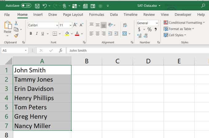
The simplest method to alphabetize in Excel is if you have one column of data. For example, if you have a column with a list of names.
- Select the column of data.
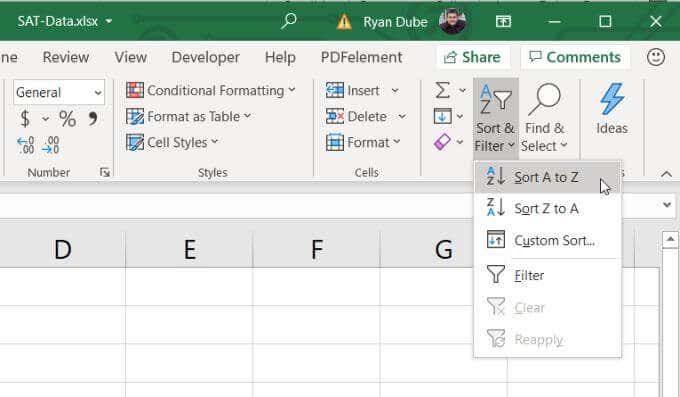
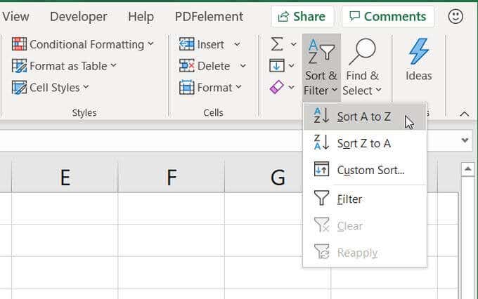
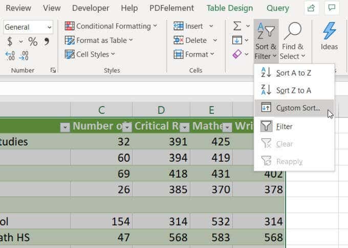
- Select the Home menu, and select the Sort & Filter dropdown in the Editing group on the ribbon.
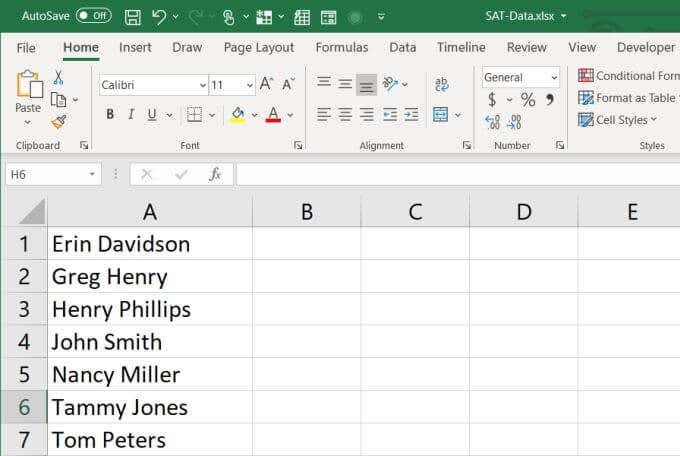
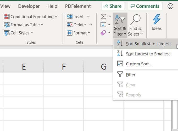
- Select either Sort A to Z or Sort Z to A depending how you’d like to organize the data. Now, when you look back at the column you highlighted, you’ll see that the data there has been sorted alphabetically using the method you chose. What if your data has numbers? For example, let’s say you have a second column with the ages of each person. You want to sort that column, so you follow the same procedure as above and select the column of data. This time, when you select Sort & Filter on the ribbon, you’ll see that the selections for how to sort have changed. These options will either sort the numbers from the smallest number to the largest, or the other way around.
Multi-Column Sorting
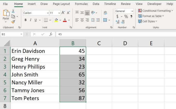
There is one problem with sorting columns individually in a table that contains multiple columns of data. If you only select one column and sort it, the other columns stay in place. This means your spreadsheet would get all mixed up and the data would no longer make sense. The answer to this is to sort all of the columns at once. Let’s do this again with the name and age example spreadsheet.
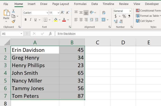
- This time, instead of selecting a single column, select the entire table.
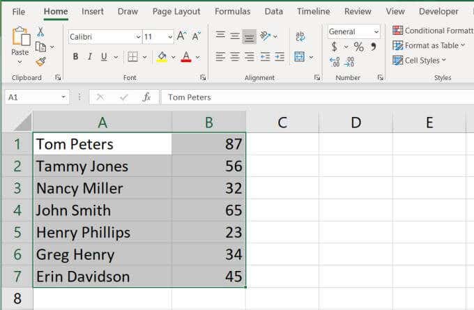
- In the Home menu, select Sort & Filter, and just as before, select your sort preference. Now, you’ll see that not only have the names been sorted alphabetically in your Excel spreadsheet, but the associated ages from the second column sorted along with them. Those ages stayed with the correct name. This works not only with a two column spreadsheet in Excel, but it’ll work regardless how large your spreadsheet is, so long as you select all of the data in the sheet before sorting. If you wanted to, you could also sort multiple columns into one, and then sort that single column instead.
Custom Sort
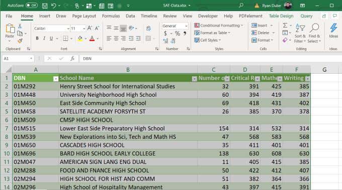
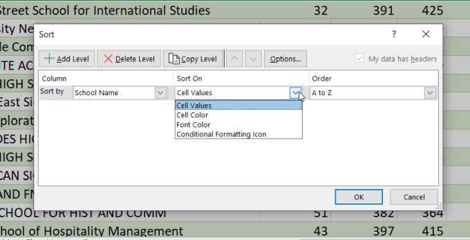
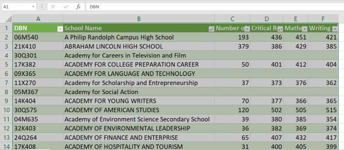
You’ll notice another option in the Sort & Filter dropdown menu is the Custom Sort. To see how this works, let’s take a much larger spreadsheet as an example. The spreadsheet in this example is a list of SAT scores for high schools in the state of New York. 2. You’ll see a new pop-up appear where you can select how each column is specifically sorted. Select the column you want to sort by, select how you want to sort it, and then select how you want to sort it (A to Z, Z to A, or Custom). You’ll notice there are some interesting Sort On choices. These are:
Cell Values: Sort alphabetically, or in the case of numbers, from low to high or high to lowCell Color: Organize data grouped by cell colorFont Color: Organize data grouped by font colorConditional Formatting Icon: Organize data by the icon in the cell from its conditional formatting logic
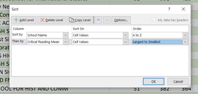
This will sort the entire table of data by the first column you’ve selected. But you can also do a secondary sort (once the first selected column is sorted). Just select Add Level. From the new fields that appear, select the Column, Sort On, and Order dropdowns again as desired. Select OK and you’ll see your entire table is now sorted by multiple columns. It’ll sort first by the initial column you selected, then the second, the third, and so on. Note: You might have noticed that the column sort options in the dropdown above included the header names rather than letters. This is because the checkbox next to My data has headers in the sort window is selected. If your spreadsheet does have headers, make sure to select this.
Alphabetize In Excel With Filter
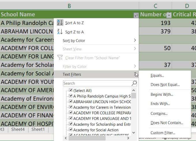
While using the Sort & Filter dropdown in the Home menu, you might have noticed there’s also a Filter option. If you select this, you’ll notice dropdown arrows appear at the top of each column. When you select one of the arrows at the top of any of those columns, you’ll see a long list of options. Here is how each of these options works:
Sort A to Z or Sort Z to A: Sort the sheet using this column alphabetically in either direction.Sort by Color: This will bring up the same multi-column sort window as in the last section above.
The other filtering options at the bottom won’t help you to alphabetize in Excel, but there are lots of options to filter out data you don’t care about. When you select Text Filters, you can choose to only display data in the sheet that:
Equals a specific valueDoes Not Equal a specific valueBegins With a word or numberEnds With a word or numberContains a word or numberDoes Not Contain a word or numberCustom Filter lets you combine any of the filters above to use multiple filters
As you can see, there are a lot of ways to alphabetize (or order numbers) in Excel. The option you choose really depends how much data you want to sort, how large the table is that you want to sort, and whether you want to sort by only one column or row, or multiple ones. Learn more about different tips and tricks for Excel, and share any other techniques you know about to sort your rows and columns in Excel.
